Increasing the Interoperability of an Earth System Model:
Atmospheric-Ocean Dynamics and Tracer Transports
NCC4-624
Milestone C: FY03 Annual Report
February 2003 – March 2004
1. Project Objectives
The objectives of this project are twofold:
1.1 Demonstrate
interoperability at the model level using the ESM (Earth System Model)
Framework (ESMF). Build a
demonstration ESM using the AGCM/OGCM and/or components developed by other
modeling teams supported by this CAN.
1.2 Estimate
the sensitivity of simulated El Niño/Southern Oscillation structures to
different background states of the coupled ocean-atmosphere system, including
testing the impact of NASA data in improving El Niño predictions.
2.
Approach
For
Objective 1.1, the approach is based on designing interfaces between the ESMF
and an expanded version of the UCLA ESM, including components developed by
other groups. Towards this objective, C. Roberto Mechoso (PI) and Joseph Spahr
visited Cecelia Deluca and members of the ESMF Development Team at NCAR on November
20 and 21, 2003, in order to discuss issues related to the ESM codes and their
future interface to the ESMF.
The sensitivity study referred to in Objective 1.2 will be performed with the UCLA AGCM/LANL POP combination, and the testing with UCLA AGCM/MIT OGCM combination. The latter will build on work at the JPL Ocean Data Assimilation Project. John Baumgardner (co-PI) is part of the team at LANL that develops the POP version with a hybrid vertical coordinate (HYPOP). Dimitris Menemenlis (Co-PI) contributes his expertise with the MIT OGCM.
3. Scientific Accomplishments
3.1 Coupling of the UCLA AGCM and MIT OGCM
The UCLA AGCM has been coupled to the MIT OGCM and a number of test integrations have been carried out both in coarse resolution and in high-resolution configurations.
The coarse-resolution UCLA AGCM (version 7.2p) is global, has 16 vertical levels, and the horizontal grid spacing is 5 deg. lon x 4 deg. lat. The high-resolution AGCM has 30 vertical levels and the horizontal grid spacing is 2.5 deg. long. x 2 deg. lat. The coarse-resolution MIT OGCM (version release1) spans 80S to 80N, has 15 vertical levels, and the horizontal grid spacing is 4 deg. both zonally and meridionally. The high-resolution OGCM spans 73S to 73N and it has 46 vertical levels. The horizontal grid spacing is 1 deg. in longitude. Meridionally, the grid spacing is also 1 deg. outside the tropics but decreases to 1/3 deg. near the Equator for improved resolution of equatorial processes. The model configuration is the same as that used for quasi-real-time ocean circulation analyses by the ECCO consortium (http://ecco.jpl.nasa.gov/external/).
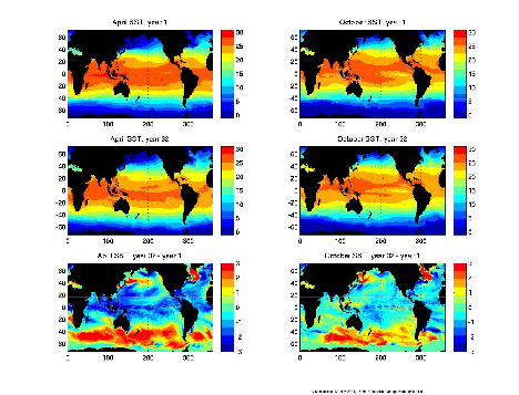
Figure 1. Monthly-mean simulated SSTs (C) for April (left column) and October (right column) at the beginning (year 1, top row) and end (year 32, middle row) of the simulation performed, and their difference (bottom row)
Figure 1 shows the monthly-mean simulated SSTs for April and October at the beginning (year 1) and end of the simulation performed (year 32). The results are encouraging with a much better developed equatorial cold tongue in October than in April, as in the observation. The development of a cold bias is evident in the tropics while a warm bias develops in the high latitudes of the Southern Hemisphere.
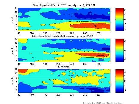
Figure 2. Deviations from the annual mean of the monthly-mean simulated SSTs (C) for at the beginning (year 1, top panel) and end (year 32, middle panel) of the simulation performed, and their difference (bottom panel)
Figure 2 shows the seasonal cycle (annual mean removed) at the equator simulated by the model at the beginning and end of the simulation, as well as the difference between these two fields. There is a clear dominance of the annual component at the beginning (as observed). Later in the simulation, a semiannual component appears.
We have verified that the model produces a significant interannual variability. Nevertheless, a time series analysis for a selected location on the equator (Nino 3) reveals that the dominant signal has a quasi-biennial period, and a smaller peak in the quasi-quadrennial periods (ENSO).
3.2 Upgrade of the PBL parameterization
The parameterization of the
planetary boundary layer (PBL) used in the AGCM was upgraded to a version with
multiple layers without loss of performance compared to the one in Milestone
E. Scaling curves were provided
and the documented source code was made publicly available via the Web.
In
the UCLA Earth System Model (ESM) version with which we started this project,
the atmospheric component (UCLA atmospheric general circulation model, AGCM)
includes a variant of the bulk parameterization for the variable-depth PBL
processes proposed by Deardorff (1972).
This is relatively simpler and physically realistic. In the model, the layer next to the lower
boundary is designated as the variable-depth PBL and is assumed to act as a
well-mixed layer (Suarez et al. 1983).
Unlike
the single-layer approach, the hybrid multi-layer parameterization allows for
vertical shears and deviations from well-mixed profiles within the PBL. These deviations are expected to be
small for thermodynamic conservative variables on a convectively active PBL,
while they can be significantly large for a convectively inactive PBL. The formulation
of processes highly concentrated near the PBL top remains tractable in this
approach, while it is more directly applicable to a variety of PBL regimes,
particularly the diurnally changing PBL over land.
The
single and multiple layer PBL parameterizations appear as options to be set up
at run time. The component of the
code directly affected by the changes is AGCM-Dynamics. The AGCM-Physics part
of the code is unchanged. A composite single layer PBL is computed from the
multilayer PBL, and computation of physical column processes other than those
of the PBL takes place as before.
Figure
3 shows the simulated January-mean precipitation, which compares reasonably
well with the observed distribution.

Figure 3: January mean precipitation simulated using the multilayer PBL. Contour interval is 2mm/day
3.3 Development of HYPOP
HYPOP is a next-generation global ocean model that features an arbitrary Lagrangian-Eulerian (ALE) treatment in the vertical grid direction. This feature allows the computational grid to conform to potential density surfaces in the deeper ocean while simultaneously resolving the mixed layer near the ocean surface with horizontal layers of nearly uniform thickness. Such treatment promises to reduce significantly the spurious vertical diffusion inherent in current generation Eulerian ocean models that use uniform thickness layers throughout the ocean volume.
Considerable effort was invested this year in development of a robust algorithm for splitting the fast barotropic motion, corresponding to external gravity wave oscillations, from the remaining slower ocean dynamics in the context of a two time level time stepping approach that is stable and robust for the strong (unsmoothed) topographical variations present in the Earth's ocean basins. Our scheme bears close resemblance to the predictor-corrector method of Higdon [JCP, 177, 59-94, 2002], but is more efficient in that it requires only one integration of the barotropic equations over each baroclinic interval. Like Higdon's, our scheme uses a subcycling approach with a small time step to advance the 2D barotropic system of equations. In slight contrast to Higdon's method, we use total velocity in the layer equations instead of baroclinic velocity. Also, to enforce consistency between the barotropic solution and the remaining slower dynamics we require the sum of the lateral fluxes over all the vertical layers to match the time-integrated lateral fluxes from the barotropic solution.
The new splitting/time stepping method has been tested against the Eulerian fixed z-level POP model using real ocean bottom topography and observed wind forcing and shown to yield stable behavior and similar results for multi-year integrations. In terms of ease of coupling to other climate model components, the two time level HYPOP formulation is simpler than the leapfrog formulation currently employed in POP.
4. Technology Accomplishments
4.1 The DDB code was upgraded and further developed
The
DDB, which was developed in Round 2, is a general-purpose tool for coupling
multiple, possibly heterogeneous, parallel models. Using the DDB, each producer sends data directly to each
consume. This strategy conserves
bandwidth, reduces memory requirements, and minimizes the delay that would
otherwise occur if a centralized element were to reassemble each of the fields
and retransmit them.
The following is a list of DDB code upgrades performed for
Milestone I:
a.
Support
both PVM and MPI communications.
b.
The
DDB checks the input arguments for consistency and valid range.
c.
The
DDB configured meta-machine and data flow matrix can be verified at the end of
registration.
d.
Modified
portions of the code to enhance code documentation, remove errors, zero out
created control data structures, and clarified DDB diagnostic output.
e.
Support
for 32 and 64 bit addressing modes.
f.
Simplified
user interface.
g.
Revised
documentation.
4.2 Software Management
The UCLA AGCM and POP versions used in this project are now managed using the tool Concurrent Versions System (CVS) and are installed in CVS repositories at UCLA(http://). The MIT GCM, including the modifications for coupling it to the UCLA atmosphere model, is also being maintained on CVS servers, both at JPL and at MIT. The MIT server (http://mitgcm.org/cgi-bin/cvsweb.cgi/MITgcm/) is configured as an anonymous CVS server, hence making the code modifications and updates publicly available in real time.
4.5 Project website
The project website was developed and is frequently updated (www.atmos.ucla.edu/~mechoso/esm). Milestone reports are posted in the website.
5. Status/Plans
We are currently working on improving the promising results obtained with the UCLA AGCM coupled to the MIT OGCM. Specifically, we are using in the AGCM the upgraded PBL parameterization described in the next sub-section of this report. This is an important task in view of the El Niño predictability studies to be performed in the third and last year of the project.
In regard to HYPOP, current effort is focused on evaluating various candidate methods for specifying the grid in the vertical direction to minimize overall numerical error. Although all the candidate methods yield almost isopycnal treatment in the deep ocean and almost uniform horizontal layers near the ocean surface where wind stress causes strong mixing, they differ in how they handle the region in between. While an abrupt transition from horizontal layers in the mixed layer to nearly isopycnal layers below the mixed layer might seem to be a simple and plausible approach, steeply plunging layer geometry typically leads to large horizontal pressure gradient errors while large layer thicknesses that frequently arise imply locally poor vertical resolution and hence significant discretization error. Therefore, some appropriate amount of horizontal smoothing of the grid is essential. However, identifying nearly optimal strategies for minimizing overall error is currently a challenging research question. Regardless of the strategy selected, it is essential the method be robust, especially at high spatial resolution. We expect our own evaluation process to be completed soon. We are also well under way in our effort to create a version of HYPOP that is ESMF compliant to meet the requirements of this project.
Work has started on the development of a conceptual model of the ESM embedded in the ESMF.
6. Point of contact
C. Roberto Mechoso
Department of Atmospheric Sciences
UCLA Mail Code 156505
405 Hilgard Avenue
Los Angeles, California 90095
7. Captions for the Graphics
Figure 1. Monthly-mean simulated SSTs (C) for April (left column) and October (right column) at the beginning (year 1, top row) and end (year 32, middle row) of the simulation performed, and their difference (bottom row)
Figure 2. Deviations from the annual mean of the monthly-mean simulated SSTs (C) for at the beginning (year 1, top panel) and end (year 32, middle panel) of the simulation performed, and their difference (bottom panel)
Figure 3: January mean precipitation simulated using the multilayer PBL. Contour interval is 2mm/day
8. Publications
None
9. Conference Presentations
The UCLA Earth System Model: Applications and Further Developments (with J. D. Farrara and D. S. Katz). General Assembly of the International Union of Geodesics and Geophysics, 30 June – 11 July 11 2003, Sapporo, Japan.
Earth system modeling at UCLA. Computers in Atmospheric Sciences (CAS) 2003 Meeting, 8-11 September 2003, Annecy, France.
10. Graduate Students and Post Docs
Gabriel Cazes – Graduate Researcher
Heng Xiao – Graduate Student