A collection of animations constructed specifically for Honors 98 (Severe Weather). The movies are either animated GIFs for QuickTime movies. The QuickTime software can be found here. File sizes for the animations are listed; some of the animations are large.
Index to this page:
|
Simulations of convective
rolls
|
Numerical simulation of boundary layer horizontal convective rolls
(HCRs). Horizontal panel shows vertical motion at 250 m above ground
level along with temperature departures (reds are warm) from the horizontal
average. Vertical cross-section shown at right. Clicking on either image
spawns 1.9 MB animated GIF in new window. Although the simulation starts
with surface heating that varies in a spatially random way, the vertical
wind shear causes coherent roll-type circulations to form.
Source: after Fovell
and Dailey (2001)
| Horizontal plane (250 m above ground) |
Vertical plane |
 |
 |
As seen in a sophisticated mesoscale model:
The summer season sea and land breezes in Southern California
sometimes result in the formation of cyclonic flow (the Catalina eddy)
over the bight, as seen in this picture of ground-surface temperature and
near-surface winds forecasted for 10Z (3 AM) 9 June, 2002. Clicking on
image spawns a 1.3 MB GIF animation spanning 48 hours and showing the
formation of Catalina eddies on successive days. Source:
R. Fovell, UCLA; made with the MM5 model

This much simpler model of the sea and land breeze still captures
many of the circulation's salient features. This is a two dimensional
model showing vertical cross-sections of
temperature perturbation (reds are warm) and vertical
velocity at left, and pressure perturbation (blues are low) and horizontal
velocity at right. The time shown is 6 PM local; the domain is 8 km deep
and several hundred kilometers wide.
Clicking on the image
spawns a 1.7 MB QuickTime movie spanning two days. Source:
R. Fovell, UCLA, using Rotunno's (1983) heating function
Initiation of convection in Oklahoma and Kansas on 12-13 June
2002. Visible satellite imagery. Click on image to spawn 2.3 MB GIF
animation in new window. Source: NCAR JOSS
Initiation of convection by/at the sea-breeze front in Florida on 11
June 1997. Visible satellite imagery. Click on image to spawn 688 KB GIF
animation in new window. Source: Unidata
Initiation of convection by/at the sea-breeze front in Florida on 2 July
1995. Visible satellite imagery. At the earliest time, rolls are
ubiquitous over the land surface (see, especially, inside red circle) and
convection has begun firing along the sea-breeze front (white arrow).
Convection
is well-developed in center and right images; note outflow boundary in
latter (red arrow). Click on any image to spawn a 1.3 MB
QuickTime movie. Source: NASA
Simulation of convective initiation involving the sea-breeze and
convective rolls: This is a vertical cross-section (60 km wide and 8
km deep) from a relatively
simple
three-dimensional model including both the sea-breeze and convective roll
simulations. The sea-breeze front (SBF) marks the marine air boundary and
a roll updraft located farther
inland. As the SBF approaches the roll, deep convection is spawned.
Clicking on the image spawns a 1 MB QuickTime animation. Look for the
significant speed variations in the SBF; it both accelerates and slows
during the period covered. Source: R. Fovell, UCLA, after Fovell
and Dailey (2001)
Squall line extending from Kansas to Texas on 7-8 May 1995.
Composite radar imagery. Note propagation to the east, development of
extended area of light precipitation on west (back) side, and development
of new convection ahead of the line. Click on image to spawn 2 MB GIF
animation in new window. Source: A. Kankiewicz, Colorado
State Univ.
Numerical simulation of a multicellular squall line. Contours:
vertical velocity; shaded: equivalent potential temperature. Note
periodic development and rearward propagation of convective cells. Click
on image to spawn 160 KB GIF animation in new window. Source:
after Fovell and Tan (1998); made with the ARPS model
Numerical simulation of stratospheric gravity waves. The
sequential development of convective
cells results in a periodic disturbance of the overlying stable
stratosphere, resulting in the generation of gravity waves (buoyancy
oscillations). Vertical velocity contoured; temperature perturbations
colored (warmed air in red). Click on image to spawn 748 KB GIF animation.
Source:
after Fovell, Durran and Holton (1992); made with the ARPS model
Effect of the subcloud cold pool on convection, part I. Image below shows a
nonprecipitating
storm in an environment with deep vertical wind shear. The storm leans
"downshear", as expected. Such a storm would precipitate into its own
inflow. Contoured: horizontal velocity; shaded:
vertical velocity (upward motion in red). Click on image to spawn a 212
KB GIF animation in new window. Source: R. Fovell, UCLA
Effect of the subcloud cold pool on convection, part II. Subcloud
cooling comes from evaporation of hydrometerors falling from the cloud.
This cooling exerts a first-order effect on storm strength andf structure.
Simulation
at left is the control run, a mature multicellular storm with "upshear"-tilting
circulation. The simulation at right shows how the control storm changes
after deactivation of subcloud cooling. Clicking on either image spawns an
872 KB GIF animation. Note the storms start with precisely the same
initial conditions. Source: R. Fovell, UCLA
| Control simulation |
Subcloud cooling deactivated |
 |
 |
|
Supercell storms and storm
splitting
|
Rotating supercell storms are favored by environments having considerable
vertical wind shear, and can form as a result of the splitting of
preexisting convection. The simulation at left had only vertical wind
speed shear. The original convective cell split into two new storms of equal strength but
having opposite senses of
rotation and very different trajectories. With directional shear (picture
at right), one of
the split storms is definitely favored. The reddish area is a rainwater
isosurface and vectors indicate midtropospheric wind perturbations.
Clicking on images spawn approximately 525 KB
QuickTime movies.
Source: R. Fovell, UCLA; made with the ARPS model
| No directional vertical wind shear |
With directional vertical wind shear |
 |
 |
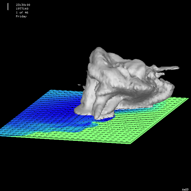
Two views of a supercell. Both panels show surface temperature (colored) with near-surface winds. Left panel depicts 0.6 g/kg condensed water isosurface; right image presents isosurface of 20 m/s updraft velocity. Clicking on the image below spawns ~ 1.5 MB animated GIFs.
Source: R. Fovell, UCLA; made with the ARPS model
| Condensed water isosurface |
Updraft isosurface |
 |
 |
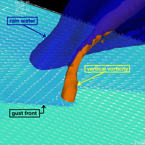
Tornado? The image below zooms in on the lower portion of the rotating supercell storm shown above. The gust front is seen in both the surface temperature perturbation and surface wind field. The blue isosurface shows a envelope of rainwater; the orange isosurface encloses areas of large cyclonic vertical vorticity. Such vertically oriented vortex tubes develop sequentially along the gust front, growing out of low-level rotation, and build upwards towards the cloud. Clicking on the image below spawns a QuickTime movie; this movie is 5 MB.
Source: R. Fovell, UCLA; made with the ARPS model
Hurricane Lili, 2-4 October 2002. Shown are enhanced IR and radar
imagery and surface map for approximately 9Z (4 AM CDT) on October 3rd.
Clicking on images spawn 2.8, 1
and 0.5 MB GIF animations in new windows. Sources: Enhanced IR
and radar imagery from Unisys; surface maps from NCEP
| Enhanced IR |
Radar |
Surface map |
 |
 |
 |
Two simulations of Hurricane Lili: At left, winds at 10 m along with
estimated radar reflectivity at 14Z (9 AM CDT) for an MM5 simulation.
Click on image to spawn a 664 Kb GIF animation. Right panel juxtaposes
COAMPS and MM5 simulations, also at 14Z. Shown are winds at 4.5 km and
cloud water field at 4 km. Clicking on image spawns 1.7 MB QuickTime
movie. Note landfall is delayed for both simulated storms and storm track
for MM5 simulation is less accurate. MM5 run also places largest
precipitation in wrong quadrant.Source: R. Fovell,
UCLA
| MM5 |
COAMPS vs. MM5 |
 |
 |
|
Downslope winds and hydraulic
jumps
|
Hydraulic jumps: Under certain conditions, air flowing over a
mountain can be accelerated on the lee slope, resulting in very strong
winds concentrated near the ground surface. The fluid there thins, as
evidenced by the colored (potential temperature) field in the left-hand
plot. Further downstream, however, the fluid can very suddenly become much
thicker in an abrupt "hydraulic jump". The jump is very turbulent. The
right-hand panel shows horizontal velocity perturbations zoomed in on the
mountain. Clicking on the images spawns 396 and 224 KB GIF animations.
Source: R. Fovell, UCLA; made with ARPS model
| Potential temperature field |
Horizontal velocity perturbation field |
 |
 |
Santa Ana winds in the Los Angeles basin are common in winter when
high pressure builds in the cold high desert. The figure below shows
surface temperature (colored) and 10 m wind vectors at 11Z (3 AM PST) for
the
January 6, 2003, high wind event. Clicking on the image spawns a 1.6 MB
GIF animation. More on Santa Ana winds may be found at this link. Source: R. Fovell, UCLA; made with
the MM5 model